To simplify things, we'll start with a 2d case (i.e., a quadtree) and extend to 3 dimensions.
A ray is defined as the vector pair (o,d). "o" is the origin, and "d" is the normalized direction vector. Any 2d point lying on the ray is defined in terms of the parametric function [x(t), y(t)]
x(t) = o.x + t * d.x
y(t) = o.y + t * d.y,
t >= 0
For a given node in the quadtree, q, we really only need to know its minimum and maximum extents since it is given that it is an axis-aligned square. This amounts to the upper left corner (x0, y0) and the lower right corner (x1, y1). In a formal sense, any node, q, is defined as the set of all points in the range --
x0(q) <= x < x1(q)
y0(q) <= y < y1(q)
The functions x0, x1, y0, and y1, give us the ranges for a quadtree. In actual implementation, we would most likely just store these ranges in a node rather than compute them with a function. From these two definitions, we can say that the ray intersects the node iff there exists one positive real-valued t such that --
x0(q) <= x(t) < x1(q) AND y0(q) <= y(t) < y1(q)
In the general implementation, let's first assume that we can project the ray along its direction to reach the limits of the node. That is, we cast the ray for some t until its x value reaches x0(q), and again for x1(q). Similarly we do this for the y limits y0, and y1.
Let's say that tx0, tx1, etc. define the values of t, such that the
ray is projected to x0, x1, etc. respectively.
This means that for node q, and ray r = (o, d) --
tx0(q,r) = (x0(q) - o.x) / d.x
tx1(q,r) = (x1(q) - o.x) / d.x
ty0(q,r) = (y0(q) - o.y) / d.y
ty1(q,r) = (y1(q) - o.y) / d.y
With this, we can say that the ray intersects the node iff there exists some t >= 0, such that --
tx0(q,r) <= t < tx1(q,r) AND ty0(q,r) <= t < ty1(q,r).
Some people have emailed me that they get a little confused here, but let me make it clear that this means for a particular value of t that satisfies BOTH conditions must exist for an intersection to exist. A simpler way to put this would be to say that we have two intervals [tx0, tx1) and [ty0, ty1). If these two intervals intersect (i.e., share a common range), and the intersection contains positive valued t's, then an intersection occurs.
This can be further simplified in implementation to say --
tmin = max(tx0(q,r), ty0(q,r))
tmax = min(tx1(q,r), ty1(q,r))
if (tmin < tmax), then an intersection occurs.
Again, assuming that positive values of t are contained in the interval [tmin, tmax]. In a simple implementation, we can prevent any negatives by simply replacing any negative values in interval computation with zeroes. By doing this, we can only have positive values in intervals if any intervals exist. If tmin = tmax, what we would likely have would be intersection in the negative direction (assuming you're cutting out negatives and replacing with zeroes, so that tmin = tmax = 0), or intersection with the node at a single point (tmin = tmax > 0). Passing through a vertex of the node isn't a very meaningful intersection unless you have an object that also passes through that node vertex. While this is a realistically possible pitfall, it would really be a very rare coincidental problem. And the cost of processing objects in the extra nodes is probably not worth it. Effectively, this shows us how to determine intersection for a given node. If the node is not a leaf, we continue further down and check its children. While you would have to check all 4 children for intersection, at the very least, you're limited only to those 4 for a given node.
Note that if you have rays that are axis aligned(1 non-zero component) or lie in an axis-aligned plane(2 non-zero components), you will simply store t-values for that particular axis (or two) that are both equal to zero for the beginning and end. Because of this, they will always be excluded from the interval of [tmin,tmax] unless no intersection actually occurs in the positive direction.
Goal
Eventually, you will generate a list of all the leaf nodes that are intersected by the ray. You can simply start by testing the ray against the root node, and if it intersects, it effectively becomes the head of a linked list. Assuming the root is not a leaf, we can then check against the 4 children of the root. Doing this, you generate a new sublist that replaces the root in this main list. Then the octree nodes pointed to by the nodes of the resulting main list have their children checked (if they're not leaves) and each of their corresponding nodes in the main list is replaced by a sublist. Of course, it's always possible to implement it without recursion, but recursion does make it simpler to follow.
More accurate to a realistic implementation of the algorithm would be that a node is checked for intersection, if it intersects, we check its children in some particular order. If the node happens to be a leaf, we add it to the list. Eventually, all the leaf nodes intersected by the ray should be present in the list, and then they can have whatever normal processing would be done (ray-object intersections and what not). At this point no further dealings with the tree itself are necessary since the list will have pointers to the appropriate nodes and their respective contents.
In extending the algorithm from quadtrees to octrees, we simply include the z component whereever needed. So for an octree node, we'd need to calculate tz0(q,r) and tz1(q,r) and so on.
In moving further down in depth of the octree, there's a simple feature of the subdivision that can be used to our advantage. That being that the children of a node are contained within the node itself. The only new subdivisions that occur are at the midplanes. That is, the set of children for a given node will also exist in the ranges [x0, x1), [y0, y1), and [z0,z1). In addition to these, there will only be one more triplet of limits to consider -- (x½, y½, z½). Rather than calculate the t-limits for a node and its 8 children (56 values), we can simply calculate all possible limits ahead of time (12 values) and use them directly to test any of the nodes. Notably, because of the fact that the midplanes are halfway along a particular axis between the near and far planes, it logically follows that the corresponding t-values themselves are halfway in between. This means that we need not explicitly calculate the mid-plane t-values because we can get them by simply averaging the t ranges of the parent. This also means that we only have to explicitly calculate the t0 and t1 values for the root node, and we can use averaging to get the appropriate values for any child.
Base algorithm Pseudocode :
assume all negative t-values are stored as zero-valued...
void ray_step( octree *o, ray *r )
{
compute tx0;
compute tx1;
compute ty0;
compute ty1;
compute tz0;
compute tz1;
proc_subtree(tx0,ty0,tz0,tx1,ty1,tz1, o->root);
}
void proc_subtree( float tx0, float ty0, float tz0,
float tx1, float ty1, float tz1,
node *n )
{
if ( !(Max(tx0,ty0,tz0) < Min(tx1,ty1,tz1)) )
return;
if (n->isLeaf)
{
addtoList(n);
return;
}
float txM = 0.5 * (tx0 + tx1);
float tyM = 0.5 * (ty0 + ty1);
float tzM = 0.5 * (tz0 + tz1);
// Note, this is based on the assumption that the
children are ordered in a particular
// manner. Different octree libraries will
have to adjust.
proc_subtree(tx0,ty0,tz0,txM,tyM,tzM,n->child[0]);
proc_subtree(tx0,ty0,tzM,txM,tyM,tz1,n->child[1]);
proc_subtree(tx0,tyM,tz0,txM,ty1,tzM,n->child[2]);
proc_subtree(tx0,tyM,tzM,txM,ty1,tz1,n->child[3]);
proc_subtree(txM,ty0,tz0,tx1,tyM,tzM,n->child[4]);
proc_subtree(txM,ty0,tzM,tx1,tyM,tz1,n->child[5]);
proc_subtree(txM,tyM,tz0,tx1,ty1,tzM,n->child[6]);
proc_subtree(txM,txM,tzM,tx1,ty1,tz1,n->child[7]);
}
While an implementation in accordance with the pseudocode above will work, there is one inefficiency that has yet to be mentioned. There is the problem that the lists that are generated are not very likely to come out sorted. While we'd have a list that contains all visited leaf nodes, the list is not sorted in order from nearest to farthest (i.e. lowest t interval to highest t interval).
There are a few ways to handle this. The simplest way is to just sort the list by t-values (thereby resulting in a list ordered nearest->farthest from the ray origin) after having generated the list. This will mean including a t-value in the list-node structure, and you can use either tmin or tmax for this. It doesn't really matter which. Somewhere in the middle as far as complications go would be to modify the addtoList function so that it inserts the selected node in the appropriate list position based on t-value. We can actually eliminate the need for a t-value in the list node structure because we can pass it into the function from proc_subtree right when it's available. The problem here is that it involves list searching and insertion for every terminal node found, which can add up to quite a big cost as the ray intersects more and more nodes. The more complicated way would be to order your testing of children in such a way that the list comes out pre-sorted. This would involve finding the entry and exit plane of a ray and modifying the order of searching based on that. While this is very much possible, it incurs an overhead of having a great deal of hard-to-predict branches. In a scene where the tree's average subdivision depth is very high, it's quite likely that post-sorting the list would be more costly than producing pre-sorted lists (the list of intersected leaf nodes would be very large). In a lower average subdivision case, the lists would probably be short enough that post-sorting the list is the smaller cost.
Determining Entry and Exit Planes
If we were to order our processing of children, we would need to know
entrance and exit planes of the ray. Fortunately, these are relatively
simple to determine. In determining tmin, we find the maximum of
the start t-values (t0's). To determine the exit plane, we simply
need know which of the 3 t0 values was the maximum.
| Maximum | Entry Plane |
| tx0 | YZ |
| ty0 | XZ |
| tz0 | XY |
Similarly for a ray exiting a node, we need to know which of the 3 t1
values was the minimum.
| Minimum | Exit Plane |
| tx1 | YZ |
| ty1 | XZ |
| tz1 | XY |
Having a way to determine entry and exit planes gives us a way to determine which of a node's children is the first one intersected as well as determine which ones are going to follow. Again, this involves some knowledge of neighbors of an octree node, but in this case, we're confined to the space of a particular parent node, and so it is no different from a SEADS table as we can simply look up the list of children. One of the greatest benefits of this is that we can avoid doing unnecessary recursive calls and only process the subtrees that are intersected without ever having to consider those that aren't.
Determining the First Node
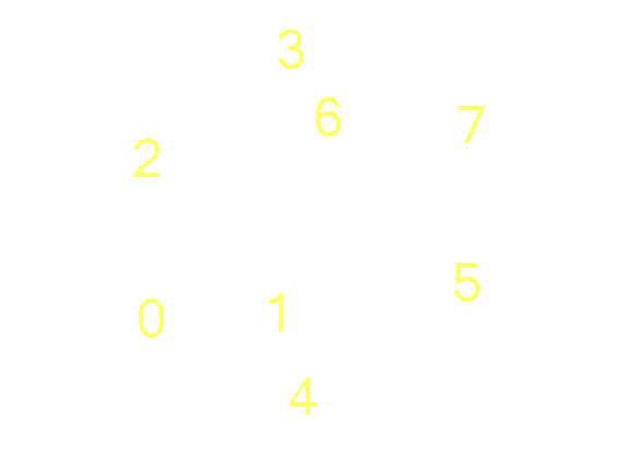
For simplicity's sake, we'll initially assume that all components of the ray direction are positive. Accounting for negative directions will be a simple extension on top of the resulting algorithm. First let's look at the ordering of our children in the octree node.
The order is not important from a theoretical point of view. It's simply important inasmuch as knowing the neighbors of a particular node and knowing which range points to which child node and so on. This is the same ordering of nodes assumed in the pseudocode earlier. Anything further will assume this ordering of children.
Once we've found the entry plane, that reduces the task to 4 possible children, with one exception. There is the fact that in assuming all our ray direction components are positive, that excludes child 7 from possibly being the first node entered. To determine the first crossed node, we further subdivide the problem using the midplanes. Quite simply, we know that tmin (whichever axis it happens to be on) is the entry point of the ray. We simply find if the midplanes are crossed before or after entry.
If we enter in the XY plane, the only possible first-intersected children
will be 0, 2, 4, and 6.
If we enter in the YZ plane, the only possible first-intersected children
will be 0, 1, 2, and 3.
If we enter in the XZ plane, the only possible first-intersected children
will be 0, 1, 4, and 5.
One of the conveniences that pops up here is that the 4 possibilities
in each case are related by 2 common bits. The XY case has numbers
using bits 1 and 2 (or no bits). The YZ case has indices using bits
0 and 1, and the indices for the XZ case use bits 0 and 2. Also,
the possibility of the first intersected child being child 0 is common
to all 3 entry planes. This can reduce the number of branches we
have for each case because we can determine the index by initially assuming
child 0 and using logical OR operations to set the correct values.
| Entry Plane | Conditions | Bit to Set |
| XY | txM < tz0
tyM < tz0 |
2
1 |
| YZ | tyM < tx0
tzM < tx0 |
1
0 |
| XZ | txM < ty0
tzM < ty0 |
2
0 |
Note that both conditions do need to be checked for any given entry plane. If they hold true, then you perform a logical OR with a bitmask for the appropriate bit.
Determining the Next Node
After determining the entry child, we also need to determine the follow
up nodes. This is done sequentially rather than trying to determine
the entire list of visited nodes at once and then processing them.
If we know which node we are in and we know the exit plane for that node,
then the appropriate neighbor is obvious. Note that the end limits
for children will include midplane t-values, but they should still be treated
as t1 values for that node. Using those, we can determine the exit
plane for a child node, and knowing which node we are in, we can determine
the next neighbor (next neighbor could potentially be nothing as we could
be leaving the parent).
| Current Sub-node | Exit Plane
YZ |
Exit Plane
XZ |
Exit Plane
XY |
| 0 | 4 | 2 | 1 |
| 1 | 5 | 3 | Exit |
| 2 | 6 | Exit | 3 |
| 3 | 7 | Exit | Exit |
| 4 | Exit | 6 | 5 |
| 5 | Exit | 7 | Exit |
| 6 | Exit | Exit | 7 |
| 7 | Exit | Exit | Exit |
So in short, in the proc_subtree function, rather than recursively calling proc_subtree for all the children, we instead have a value keeping track of the current child we are in. The initial value of this "currentChild" value is determined by finding the first intersected node. Then we recursively call on currentChild, and then follow that by determining the next node, and process that child. This goes on in a loop until currentChild is determined to be an "Exit" state.
Once again, though, the issue of axis-aligned rays rears its head. While using zero-valued constants for the start and end t-values was certainly valid when this ordered search was NOT done, it doesn't quite work out otherwise. Now we have no choice but to store positive and negative infinite values (or rather, very large magnitude values). Let's say for instance that we have a ray in the YZ plane (ray->d.x = 0). Now we have to store things a little differently. In short, we have to compare the x values against the origin x values. If the x value is greater, we store a +infinity. If it's less, we store a -infinity. Similarly, we'd have to do this for midplane tx-values. A simple way to fudge this is by simply overwriting 0's in the direction vector with some very small positive value. The value has to be sufficiently small that it won't cause any errors in node selection within the range of the object space. This also means that we can't throw out negative t-values and write them in as zeroes, and we'll now have to check intervals for negatives. When you have very large-magnitude t-values, there may be a concern that these very large t's will override the normal-range t's and corrupt the tmin and tmax used for intersection tests. Fortunately, though, such things will only happen for nodes that are NOT intersected by the ray, and the (tmin < tmax) test will give such a result. Moreover, after the initial test with the root, nodes that aren't intersected by the ray won't even be considered.
Because t-values are explicitly calculated only once, we don't need to actually overwrite any zero-values in the ray directions. This allows our ray-object intersection tests that will follow to maintain their accuracy.
As was mentioned earlier, the limited searching approach so far is based
on the assumption that all the components of the ray are positive.
In order to account for the rays that have negative components, we have
to introduce some modifications. Because the test system only works
for positive components, we have to reflect the ray about the midplane
of the octree root for that negative axis. And then we will be able
to negate the negative direction and treat it as a positive. In the
case that we have only an x-component that is negative, we do this as follows
--
ray->d.x = -(ray->d.x);
ray->o.x = octree->size - ray->o.x;
Octree->size represents the length of a side of the bounding cube that the octree resides in. If other components are also negative, we do the same for them. Also, if you implement an octree where the root bounding box is not necessarily a cube, you'd have to use the corresponding side length for the axis (in this case, sizeX).
After doing this, we would be able to perform an accurate traversal of intersections, but the labelling would be wrong for the mirrored ray. For instance, take a ray where the x-axis is negative, and the ray happens to pass through children 4, 6, and 2 (in that order). The mirrored ray would be detected as passing through 0, 2, and 6. What we'd need to do is transform the labels so that we can run the process as if the ray were passing through 0->2->6, but would actually access nodes 4->6->2. To do this we need to find a function, f(i), that will transform the indices. For example, if ray->d.x is negative, instead of having the default image order (0,1,2,3,4,5,6,7), we would have the order (4,5,6,7,0,1,2,3). If ray->d.y is negative, we'd have (2,3,0,1,6,7,4,5). If both d.x and d.y are negative, we'd have (6,7,4,5,2,3,0,1).
Fortunately, in the process of finding our entry node, another interesting convenience pops up. It shows that there is a bit corresponding to an axis. If you notice, any comparison of txM against any variable resulted in setting bit 2. Similarly, any comparison of tyM against any variable resulted in setting bit 1. Likewise, bit 0 corresponded to tzM comparisons. Conversely, wherever tx0 was the max value to compare against, there was no possibility of modifications being made to bit 2. And so on for ty0 and tz0. What this shows is that in indexing, we have bit correspondence for the axes. This means that if the ray direction is negative on the axis, we need only switch the bit corresponding to that axis. To switch the state of individual bits, we simply use the XOR operator. This results in a transformation function f(i) such that --
f(i) = i ^ a
a = 4sx + 2sy + sz, where
s# is 1 if the direction on that axis is negative, and 0 otherwise.
Note that this transformation is a method by which to "fool" the algorithm into thinking that the ray is positive in all directions. We do not change the parameters for the children that are indexed by the functions that find the appropriate nodes. We simply index a different node and pretend that it is the same one.
e.g. In the original pseudocode for processing node 2, we had proc_subtree(tx0,tyM,tz0,txM,ty1,tzM,n->child[2]).
In the modified version, we would call proc_subtree(tx0,tyM,tz0,txM,ty1,tzM,n->child[2^a]),
assuming 'a' has been determined already (and 'a' is a constant for a given
ray). Note that the algorithm never actually accesses the nodes;
it only adds them to the list to search if the node is a leaf. This
makes it possible to fool the code because it will never actually check
that it is at child[2] when it's normally supposed to be.
The apparent after-effects of our child ordering suggests that it is necessary to implement your octree library such that children are ordered as described in this tutorial. We are exploiting properties found in the current ordering scheme, but there are several possible permutations that will have the same properties (albeit with different bit correspondence).
byte a;
// In practice, it may be worth passing in the ray by value or passing
in a copy of the ray
// because of the fact the ray_step() function is destructive to the
ray data.
void ray_step( octree *o, ray *r )
{
a = 0;
if (r->d.x < 0)
{
r->o.x = o->size - r->o.x;
r->d.x = -(r->d.x);
a |= 4;
}
if (r->d.y < 0)
{
r->o.y = o->size - r->o.y;
r->d.y = -(r->d.y);
a |= 2;
}
if (r->d.z < 0)
{
r->o.z = o->size - r->o.z;
r->d.z = -(r->d.z);
a |= 1;
}
compute tx0;
compute tx1;
compute ty0;
compute ty1;
compute tz0;
compute tz1;
float tmin = Max(tx0,ty0,tz0);
float tmax = Min(tx1,ty1,tz1);
if ( (tmin < tmax) && (tmax > 0.0f) )
proc_subtree(tx0,ty0,tz0,tx1,ty1,tz1,
o->root);
}
void proc_subtree( float tx0, float ty0, float tz0,
float tx1, float ty1, float tz1,
node *n )
{
int currNode;
if ( (tx1 <= 0.0f ) || (ty1 <= 0.0f) || (tz1
<= 0.0f) )
return;
if (n->isLeaf)
{
addtoList(n);
return;
}
float txM = 0.5 * (tx0 + tx1);
float tyM = 0.5 * (ty0 + ty1);
float tzM = 0.5 * (tz0 + tz1);
// Determining the first node requires knowing which
of the t0's is the largest...
// as well as comparing the tM's of the other axes
against that largest t0.
// Hence, the function should only require the 3
t0-values and the 3 tM-values.
currNode = find_firstNode(tx0,ty0,tz0,txM,tyM,tzM);
do {
// next_Node() takes the
t1 values for a child (which may or may not have tM's of the parent)
// and determines the next
node. Rather than passing in the currNode value, we pass in possible
values
// for the next node.
A value of 8 refers to an exit from the parent.
// While having more parameters
does use more stack bandwidth, it allows for a smaller function
// with fewer branches and
less redundant code. The possibilities for the next node are passed
in
// the same respective order
as the t-values. Hence if the first parameter is found as the greatest,
the
// fourth parameter will
be the return value. If the 2nd parameter is the greatest, the 5th
will be returned, etc.
switch(currNode) {
case 0 : proc_subtree(tx0,ty0,tz0,txM,tyM,tzM,n->child[a]);
currNode = next_Node(txM,tyM,tzM,4,2,1);
break;
case 1 : proc_subtree(tx0,ty0,tzM,txM,tyM,tz1,n->child[1^a]);
currNode = next_Node(txM,tyM,tz1,5,3,8);
break;
case 2 : proc_subtree(tx0,tyM,tz0,txM,ty1,tzM,n->child[2^a]);
currNode = next_Node(txM,ty1,tzM,6,8,3);
break;
case 3 : proc_subtree(tx0,tyM,tzM,txM,ty1,tz1,n->child[3^a]);
currNode = next_Node(txM,ty1,tz1,7,8,8);
break;
case 4 : proc_subtree(txM,ty0,tz0,tx1,tyM,tzM,n->child[4^a]);
currNode = next_Node(tx1,tyM,tzM,8,6,5);
break;
case 5 : proc_subtree(txM,ty0,tzM,tx1,tyM,tz1,n->child[5^a]);
currNode = next_Node(tx1,tyM,tz1,8,7,8);
break;
case 6 : proc_subtree(txM,tyM,tz0,tx1,ty1,tzM,n->child[6^a]);
currNode = next_Node(tx1,ty1,tzM,8,8,7);
break;
case 7 : proc_subtree(txM,txM,tzM,tx1,ty1,tz1,n->child[7]);
currNode = 8;
break;
}
} while (currNode < 8);
}
Notably, the (tmin < tmax) comparison has moved from the proc_subtree() function to the ray_step() function. This is because the proc_subtree() function will only be called on nodes that are intersected, so there is no need to check the nodes for intersection after having determined it for the root.
One problem that may come up is when a ray passes through edges or vertices. The default next_node() function is not equipped to deal with anything other than face neighbors. We could potentially consider edge and vertex neighbors, but that would complicate the search for the next node, and those complications will give rise to speed problems on every call to the function. At most, edge intersection will cost nothing more than one extra node in the list. Vertex intersection will cost 2 extra nodes added to the list. This is most likely a smaller cost than having a slow function running for every recursive call. Moreover, vertex and edge intersections are fundamentally a rare occurence. They are not common enough to consider a major crippling problem.
In this aspect, the base algorithm without the ordered searching was actually advantageous. It had no weaknesses with vertex and edge neighbors and it wouldn't add unnecessary nodes to the list. This is largely because of the fact that all the children were examined for intersection and the (tmin < tmax) test was performed in the proc_subtree function. This meant that meaningless intersections would be dropped out and not added to the list. Adding the (tmin < tmax) test to the proc_subtree function in this version would work, so long as we know such skipping of nodes will not cause any problems. While there will be unnecessary recursive calls that drop out immediately, there will not be unnecessary nodes added to the list.
In summary, what results is a comprehensive and fairly elegant algorithm for ray walking through octrees of any type and of variable depth. Moreover, it can even be extended to adaptive octrees by explicitly calculating dividing plane t-values, which may not necessarily be at the halfway point. Fortunately, when it is used in an actual raytracing context, the use of ray stepping through a spatial subdivision hierarchy will give rise to better performance as depth gets higher (with diminishing returns, of course). An octree proves especially effective because it does not require a great depth to accomplish a sufficient partitioning of objects.
With the base algorithm, we have a reasonably fast approach that is almost universal in its application. Adding on the ordered searching results in an additional optimization and reduction in unnecessary calls. The number of operations is minimized because of its top-down fashion, and the use of previous stages results in each subsequent stage. It can be shown that a top-down recursive approach performs better than a DDA method primarily due to the lack of restrictions placed on the tree structure. Similarly, an octree ray traversal performs better than a BSP or kd-tree traversal when the contents of the scene are not excessively sparse. The computational cost of ray searching through a kd-tree is similar to that of searching through an adaptive octree, but the difference in depth allows the octree search to perform better overall. Only in a sparse scene would a binary tree search perform better due to its lower branching factor. This can be shown to be an artifact of using an octree itself, because of the large amount of wasted space that results in a sparse scene. Aside from performance, it also happens to be a comprehensible algorithm that is easy to implement in a rendering system.
References :
M. Agate, R.L. Grimsdale, P.F. Lister. The HERO Algorithm for Ray Tracing Octrees. Advances in Computer Graphics Hardware IV R.L. Grimsdale, W. Strasser (eds) Springer-Verlag, New York, 1991.
J. Amanatides, A.Woo. A Fast Voxel Traversal Algorithm for Ray Tracing. Eurographics87. Proceedings of the European Computer Graphics Conference and Exhibition, August 1987, pp 3-10.
J. Arvo. Linear-time voxel walking for octrees. Ray Tracing News 1(12), March 1988. Available under anonymous ftp from drizzle.cs.uoregon.edu
J. Spackman, P.J. Willis. The Smart Navigation of a Ray Through an Oct-Tree: Computer & Graphics Vol. 15(2), pp.185-194, 1991.
K. Sung. A DDA Octree Traversal Algorithm for Ray Tracing. Eurographics91.
Proceedings of the European Computer Graphics Conference and Exhibition,
F.H Post and W. Barth (eds), pp. 73-85, North Holland, 1991.