Edge-Directed Interpolation

---

Anyone who has done anything with graphics and/or image processing has had to deal with image interpolation in one way or another.  Most of the graphics coders out there have dealt not far beyond the the bilinear texture interpolation that is built into our 3d accelerator hardware.  Even so, most of us are able to recognize its weaknesses and cases where it produces quite troublesome visual cues.  Theoretically, we get some improvements in more recent video cards by virtue of anisotropic filtering.  However, anisotropic filters serve more as a "don't make it look so bad" solution rather than an "it will look good" solution.  The interpolation itself is faulty.

Well, the idea behind Edge-directed interpolation(EDI) is to use statistical sampling to ensure quality of an image when you scale it up.  This is inasmuch as scaling is used on the actual image data to interpolate to a new superresolution result as opposed to zooming in on an image, where you actually WANT to see individual pixels.  There were several earlier methods that involved detecting edges to generate blending weights for linear interpolation or classifying pixels according to their neighbour conditions and using different otherwise isotropic interpolation schemes based on the classification.

We've all seen the movies where FBI agents enhance an image so that faces can be identified and so on...  well, that's rather unrealistic, but EDI is *something* like that.  It's not going to produce features that weren't there before, but what it DOES do is maintain features that originally existed rather than making the image all blurry when it's scaled up.

The idea is to make sure that the image is NOT smooth perpendicular to edges and it IS smooth parallel to edges.  The first of the EDI algorithms developed came from Jan Allebach and Ping Wong.  While the Allebach/Wong method does accomplish the main goals of EDI, it also tends to be overly sensitive and produces noisy artifacts in the upsampled image.  A newer method came along from Xin Li and Michael Orchard which cured these problems at a minor complication cost over linear interpolation.  As I read the original paper, though, it took a little deciphering on my part as far as the equations...  Not that they were complicated;  They just suffered from poor typesetting that made most of the math look bizzare.  Ultimately, though, it works out to a least-squares approximation.

So after a little mulling, I simplified the whole thing and worked out a few optimizations as well as a handful of extensions to consider in the long run.

Let us first consider the case of scaling a grayscale image with no interpolation at all (this means not even nearest-neighbour).

The image on the left represents a 3x3 image.  Each square is a single pixel and the spaces in between them are just for illustration.  The image on the right is scaled up to 6x6 (with the last column and row cropped away to make it 5x5) with no interpolation.  That is, we have 16 more pixels in the superresolution image, but we've done nothing to give them any values, so they simply remain zero-valued.  As for the markings, the pixels marked 'a' do not have all their adjacent neighbours pre-determined.  The pixels marked 'b' have pre-existing neighbours...  they just happen to be diagonal neighbours.

Fortunately, the question of diagonal or axial neighbours makes no difference to NEDI.  Covariances can be computed for any axis orientation, so for the 'b' pixels, we simply use diagonal-axis covariances rather than xy-axis covariances.  The idea behind using covariance characters is that it gives us a relative flow of differential characteristics by which to tune the interpolator so that its support is along the edges only.  NEDI tends to preserve smoothness along edges of arbitrary orientation, and does not produce smoothness perpendicular to the edges.

In practice, we obviously wouldn't concern ourselves with NEDI over a 3x3 image.  Computing of covariances is done inside of a local window of some size, MxM.  Usually, we use at least a 4x4 window for reliable estimation of covariances.  The fundamental problem is simply taking an HxW image and scaling it to a KHxKW image.  For the sake of this document, we'll stick to a case of K=2.  For original image P, and superresolution image Q, we will simply assert that P(x,y) = Q(2x, 2y).  This will at least solve for 25% of the pixels in the raster image of Q.  For the time being, we will stick to 4th order linear interpolation in our final solution.  That is, linear interpolation with only 4 neighbours considered.  The local covariances at the high resolution level can be used to find the set of weights for optimal weighted linear interpolation according to an MSE metric.  Since we cannot directly have access to the covariances at high resolution, we instead replace it with the low resolution counterparts.

In theory, although we are sticking exclusively to the case of K=2, we can actually achieve a scaling factor for all K=2^k simply by repeating the process k times.  The only real problem with doing this is that some accuracy is lost by the nature of using integer storage for images.  If scaling a float-HDR image, this is less of a concern because of the higher precision.  In an infinite-precision-float-based image format, repetition would produce numerically identical results to special case implementations for a particular value of K, assuming we run across no sensitivity problems.  If lack of precision errors are a concern, we can always achieve a correct result by using a float image format in memory and only rounding the final result.  For cases like K=3 (that is, K not equal to a power of two), we can achieve this simply two ways.  We can use NEDI for K=2, and bilinear interpolation to upsample for K = 1.5.  The other option is to use NEDI for K = 4, and then bilinear downsampling for K = 0.75.  Obviously, the former is faster, while the latter is higher quality.

The 'b' pixels correspond to those that are at Q(2x+1, 2y+1) for the superresolution image Q, where Q(2x, 2y) = P(x,y).  By filling in the values for 'b' pixels, we end up completing the lattice for all Q(i,j), where (i+j) is even.  This leaves only the 'a' pixels which are the set of all Q(i,j), where (i+j) is odd.

To compute the ideal weights, we consider the following variables.

M -- local window of pixels is of size MxM
y -- A column vector of size M² containing the pixels in the window.  y(k) is kth pixel in the window. 
C -- A matrix of size 4xM² containing the interpolation neighbours of each pixel.  The kth row vector contains the 4 interpolating neighbour pixels of y(k).

     1                        1
R = --- * CT · C         r = --- * CT · y
    M*M                      M*M

R will end up being a 4x4 matrix, and r will be a column 4-vector.  Wiener filtering tells us that optimal MMSE linear interpolation weights can be computed using the following.

a = R-1  · r = (CT · C)-1 * (CT · y)

The resulting 4-vector, a, will contain the interpolating weights for the 4 neighbours.  These weights are simply multiplied by the corresponding neighbours and the results are summed together to generate the new pixel.  According to the paper by Li and Orchard, the weights computed by using the diagonal neighbours of P(x,y) would be the same weights used for Q(2x+1, 2y+1) ('b' pixel).  Similarly, weights computed using axial neighbours would also be used for the 'a' pixels.  The examples have been assuming a single channel so far, but the algorithm can easily be extended to color images by simply using the same process for all channels.  For obvious reasons, the process cannot be used on indexed color images for the same reasons that interpolation of any kind (excluding nearest neighbour) cannot be used on indexed color images.  Notably, there are ways to improve performance on color images than to simply apply the process once per channel on RGB color.  For instance, using images in colorspace that separates luminance and chrominance (e.g., YIQ, YUV, YCbCr) means that we can limit EDI to only one channel.  Namely, the luminance channel Y.  The chrominance channels can be handled with reasonable quality by mere bilinear or bicubic interpolation (to be accurate, this holds true for natural images, but not quite true for overtly graphical or 'cartoony' images).  RGB color would require the use of NEDI on all 3 channels because each channel controls both luminance AND chrominance simultaneously.  Similarly, in HSL colorspace, we can afford bilinear or bicubic on the H channel, but NEDI is warranted on the S and L channels.

Let's say we're scaling up an image and what we have above is some small section of the image.  Now each intersection in the graph is a pixel, and the dots are locations of new pixels in the superresolution image for which we're trying to solve.  These would be "b" pixels according to our previous diagram.  Now this 6x6 block actually corresponds to a window size of M=4.  Similarly, we'd actually need pixeldata from a 4x4 block for a window size M=2.  Let's first consider a window size of M=2, in which case the pertinent pixels are a 4x4 block in the upper left corner.  While I am numbering the pixels by their position in the subblock, it should be noted that what we'd actually use in our computations are the actual pixel values, be they RGB or grayscale or YUV or whatever.  In this case, we'll just assume that this is some section of a grayscale map and the pixel numbers are also the actual grayscale levels of the pixels.  Let's take a superresolution pixel at the purple dot's location, and use a window size of 2.

yT = [ 8 9 14 15 ]

    [ 1  3 13 15 ]
    [ 2  4 14 16 ]
C = [ 7  9 19 21 ]
    [ 8 10 20 22 ]

The 2x2 window around the new pixel includes the pixels 8, 9, 14, and 15 (I use the transpose of y to save space because it's actually a column vector).  And since we're dealing with a "b" pixel, the interpolation neighbours of consideration are the diagonal neighbours, so in the matrix C, each of the row vectors are the 4 diagonal interpolation neighbours of each of pixels in the 2x2 window.  For instance, the diagonal neighbours of pixel 8 are pixels 1, 3, 13, and 15, and so on for pixels 9, 14, and 15.

For the case of a window size of 4, we'll need the entire 6x6 block, so I'll build that example for the red dot in the diagram.  The window will include the 4*4 pixels surrounding the new superresolution pixel at the red dot's location.

yT = [ 8 9 10 11 14 15 16 17 20 21 22 23 26 27 28 29 ]

     [  1  2  3  4  7  8  9 10 13 14 15 16 19 20 21 22 ]
     [  3  4  5  6  9 10 11 12 15 16 17 18 21 22 23 24 ]
CT = [ 13 14 15 16 19 20 21 22 25 26 27 28 31 32 33 34 ]
     [ 15 16 17 18 21 22 23 24 27 28 29 30 33 34 35 36 ]

Note that I put the transpose of C here in this case to save some space.  So the aforementioned row vectors in the matrix C are column vectors this time around.  Again, we're dealing with "b" pixels, so we use the diagonal neighbours of the pixels in the window.  If we were working on "a" pixels, we'd use the axial neighbours.  For instance the axial neighbours of pixel 8 would be pixels 2, 7, 9, and 14.

As you may have guessed, using a window of size 2 is a lot faster than using a window of size 4.  Also, more importantly, with larger windows, we consider a larger neigbourhood and may lose some local characteristics -- in short, that makes for a more blurry result.  This makes it sound as if a smaller window is invariably better for NEDI.  Unfortunately, for us, with smaller windows comes more ill-conditioning of matrices, which can lead to horrific errors in generating interpolation weights.  Often times, we see this in the form of stray pixels and weird misshapenness in the resulting superresolution image.  This happens a great deal with regions that show severe gradients across edges.

The simplest is a performance-oriented variation.  Pre-computing weights for all the pixels in the window of the original image.  For M=4, we'd have 16 pixels in an MxM window.  We can pre-compute the 4-vectors of weights for both axial neighbours and diagonal neighbours for all those 16 pixels and store them ahead of time.  Even though neighbours of a pixel in a window may be outside the window doesn't really matter because we will only be considering those pixels for a given MxM block.  By doing this, we are only calculating weights for each pixel once.

Another variation is to interpolate weights.  Every pixel in the original image will generate its own set of weights based on its own local covariance.  This means that, for instance, direct replacement of the weights for Q(2x+1, 2y+1) by the weights generated for Q(2x, 2y) may not be absolutely correct.  For every pixel, you are considering 4 interpolation neighbours from which you take a weighted sum.  In theory, we can consider all 4 of those neighbours in the generation of weights.  In short, we take all the 4 interpolation neighbours and average the pre-computed set of weights to generate a local weighting.  The end result is that instead of averaging pixels, as is done in bilinear interpolation, we are averaging the covariance characters.  In this case, you would act as if the current image is a superresolution image based on a yet lower resolution image and interpolate the blendweights.

Further still, we can increase the order of the linear interpolation.  As described above, the problem simply handles things by 4th order interpolation because we're limited to scanning only 4 directions.  The only neighbours available to the high resolution image during generation are either vertex(diagonal) neighbours or edge(axial) neighbours.  However, we can potentially increase the order of interpolation by including neighbours that are farther down in those 4 directions.  For example, even though we're limited to scanning in 4 directions, we can check against 2 pixels in each direction rather than one, thereby resulting in 8th order interpolation.  One of the nice advantages of using higher order interpolation is that it naturally increases the size of the matrices involved and reduces chances of ill-conditioning without having to use larger neighbourhoods.  Of course, it's a significantly higher computational cost, for instance, to have to invert 8x8 matrices than 4x4.

original image

Scaled up 16x (4x in each axis)

Bilinear interpolation	Bicubic interpolation
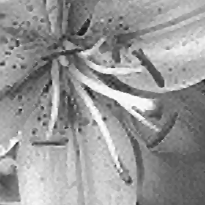
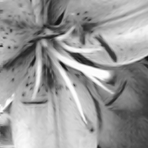
Allebach & Wong EDI	Li & Orchard New EDI